Gating, not averaging: HetMoE for transcription factor binding sites

Transcription factors are proteins that switch genes on and off by binding DNA. The stretch of DNA a factor binds is its binding site, and each factor prefers a short recurring pattern called a motif, typically 5 to 20 nucleotides long. Several factors in this study matter in cancer: FOXM1 is often overexpressed in tumors, and STAT3 dysregulation is linked to several cancers.

Convolutional models such as DeepBIND¹ predict binding sites well for the factor they were trained on, but generalize poorly to factors they have not seen. That out-of-distribution (OOD) setting, where the test factor was never in the training set, is what this paper targets. We score models with AUC (area under the ROC curve), which measures how well a model ranks bound sequences above unbound ones: 0.5 is chance and 1.0 is perfect.

In short

What we built: HetMoE, a mixture of experts that combines frozen DNA models of different architectures and learns, for each input sequence, how much to trust each one.
Headline result: on 23 held-out factors with a defined motif, HetMoE reaches a mean AUC of 0.821 ± 0.005 over three seeds, against 0.799 ± 0.008 for a fine-tuned DNABERT-6 language model.²
Where the gain comes from: per-input gating, which beats a static average of the same experts by 0.073 AUC.
Explanations: ShiftSmooth, an attribution method that averages gradients over small shifts of the input and gives more stable motif maps.

This is joint work with Ian E. Nielsen (Rowan University), and Ian and I share first authorship. I developed the methods, and together we wrote the software, curated the data and drafted the manuscript. Muhammad Umer (Fairleigh Dickinson University), Ravi P. Ramachandran (Rowan University, corresponding author) and Ghulam Rasool (Moffitt Cancer Center) co-designed and supervised the study.

Why held-out factors are hard

A sequence model for one factor learns that factor’s motif grammar and has little to go on for another. Genomic language models such as DNABERT³ aim to fill this gap with pretraining, but in a preliminary comparison on GATA3, embeddings taken directly from a pretrained DNABERT gave a lower test AUC than convolutional DeepBIND embeddings. A DNABERT-6 fine-tuned for binding-site prediction is a different matter, and it stays in the study as the strongest baseline.

The evaluation has two common traps. First, many TFBS benchmarks create negatives by dinucleotide-shuffling the positives, and a classifier trained this way can learn to spot the shuffling artifact instead of binding.⁴ Second, some factors, such as the RNA polymerase II subunit POLR2A, have no intrinsic DNA motif and are recruited through protein-protein interactions, which caps any sequence-only prediction. Pooling them with motif-rich factors blurs what the average measures.

How it works

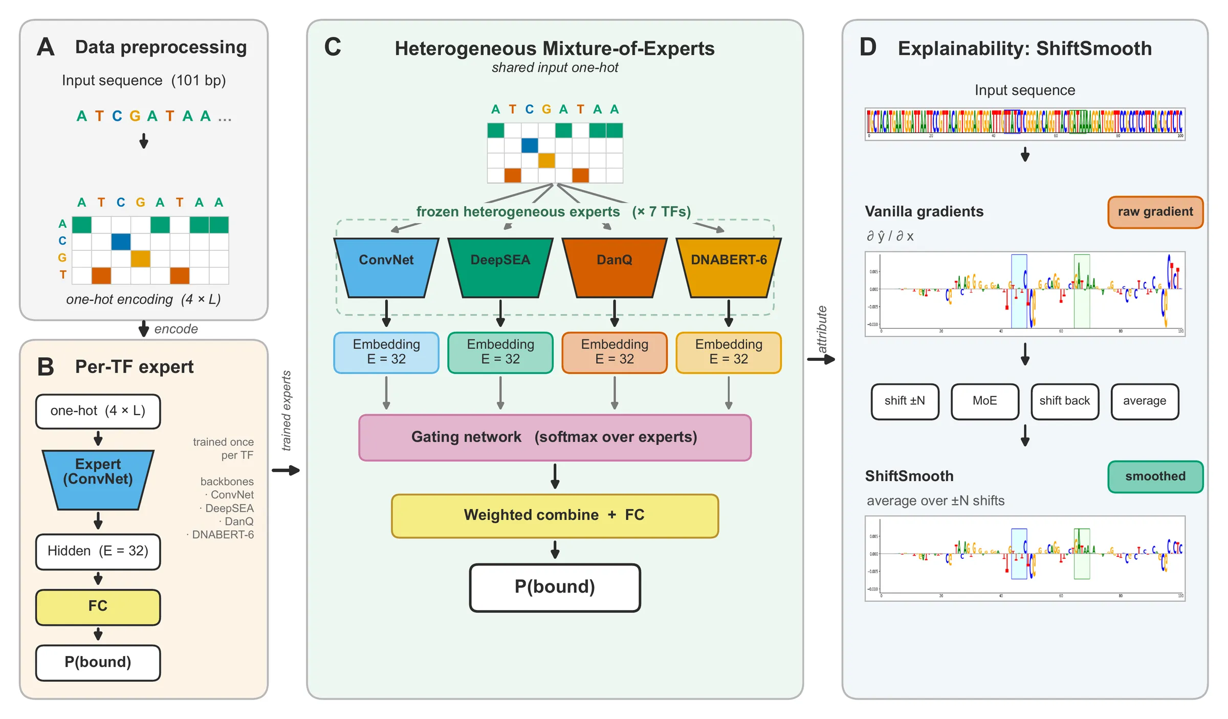
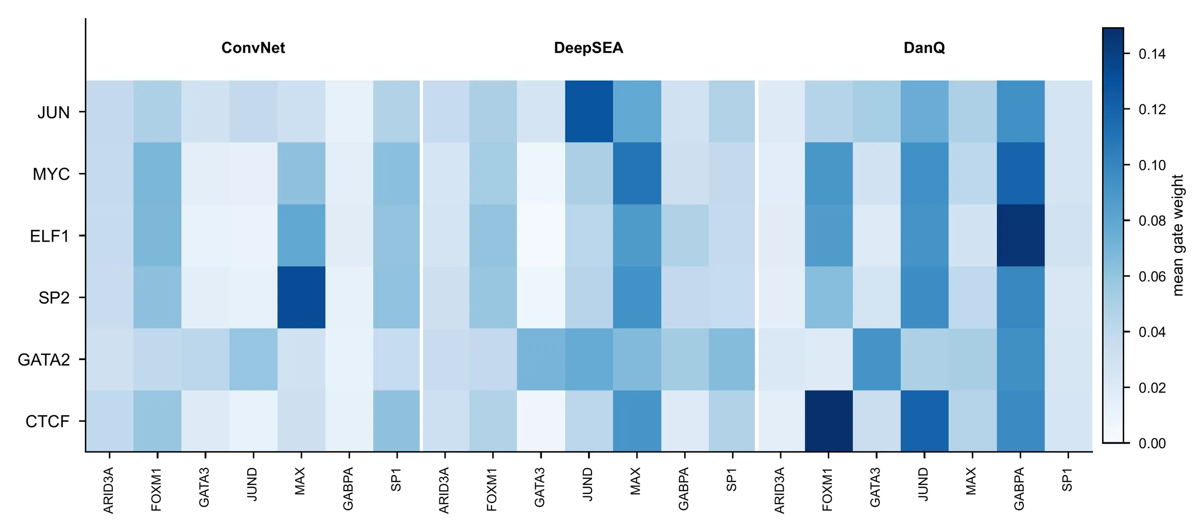
A mixture of experts is a set of models (the experts) plus a gating network that decides how much each one contributes to a given input. HetMoE is a dense mixture: every frozen expert processes every input, and the gate learns input-dependent softmax weights over their 32-dimensional embeddings. A sparse mixture would instead route each input to a few experts.

Unlike weighted averaging or bagging, the weights change with every input. Unlike stacking, the gate combines internal embeddings, not final predictions. Because the gate only sees embeddings, the experts need not share an architecture, which is what makes the pool heterogeneous.

Experts as embedding producers

The base expert is a modified DeepBIND convolutional network. Its pooling type (max, or max plus average) is chosen by Optuna hyperparameter search, and a new linear layer projects pooled features to a 32-dimensional embedding, followed by layer normalization so no expert dominates the gate through scale alone. DeepSEA⁵ and DanQ trunks enter as frozen feature extractors with a lightweight linear probe (Linear plus LayerNorm) onto the same 32-dimensional space. DNABERT-6 embeddings, built from overlapping 6-mer tokens, are precomputed once, so the gate trains the same way whatever the expert type.

Ablations on a convolutional reference pool support two choices. Changing the embedding size across $E \in \{16, 32, 64, 128\}$ moves the OOD mean by less than 0.01 AUC, so we keep $E = 32$ as a balance between capacity and cost. Freezing the experts matches fine-tuning to within bootstrap noise, and mixture training takes 5.5 s with 3,492 trainable parameters instead of 497.7 s with 11,047.

The gate

With $N_e$ experts producing embeddings $e_i$ , each embedding is first mapped by a per-expert linear projection to $h_i$ . The concatenated embeddings $\mathbf{E} = [e_1, \dots, e_{N_e}]$ drive the gate, and the prediction is a gated sum:

\alpha = \mathrm{softmax}\!\left(\mathbf{E}\,W_{\text{gate}} + b_{\text{gate}}\right), \qquad m = \sum_{i=1}^{N_e} \alpha_{:,i} \odot h_i, \qquad \hat{y} = \sigma\!\left(m\,W_{\text{class}} + b_{\text{class}}\right)

The per-expert projections, the gate and the classifier are the only parameters learned at this stage. They are trained with SGD and Nesterov momentum (learning rate 0.01, momentum 0.98, batch size 256), with early stopping on in-distribution validation AUC. Two stabilizers keep the mixture from collapsing: each expert’s embedding block is L2-normalized before the gate, and a gate-entropy term with coefficient $10^{-3}$ is added to the binary cross-entropy loss.

ShiftSmooth

Attribution methods explain a prediction by scoring how much each input position contributed to it; for DNA, the scores are drawn as a sequence logo. SmoothGrad⁶ reduces attribution noise by averaging gradients over Gaussian-noised copies of an image. That does not carry over to DNA: a one-hot nucleotide plus Gaussian noise is no longer a nucleotide. What does vary in genomic data is the window, whose start and end are somewhat arbitrary within a few bases. ShiftSmooth therefore circularly shifts the input by $n$ positions, takes the gradient of the class score, shifts that gradient back into register and averages:

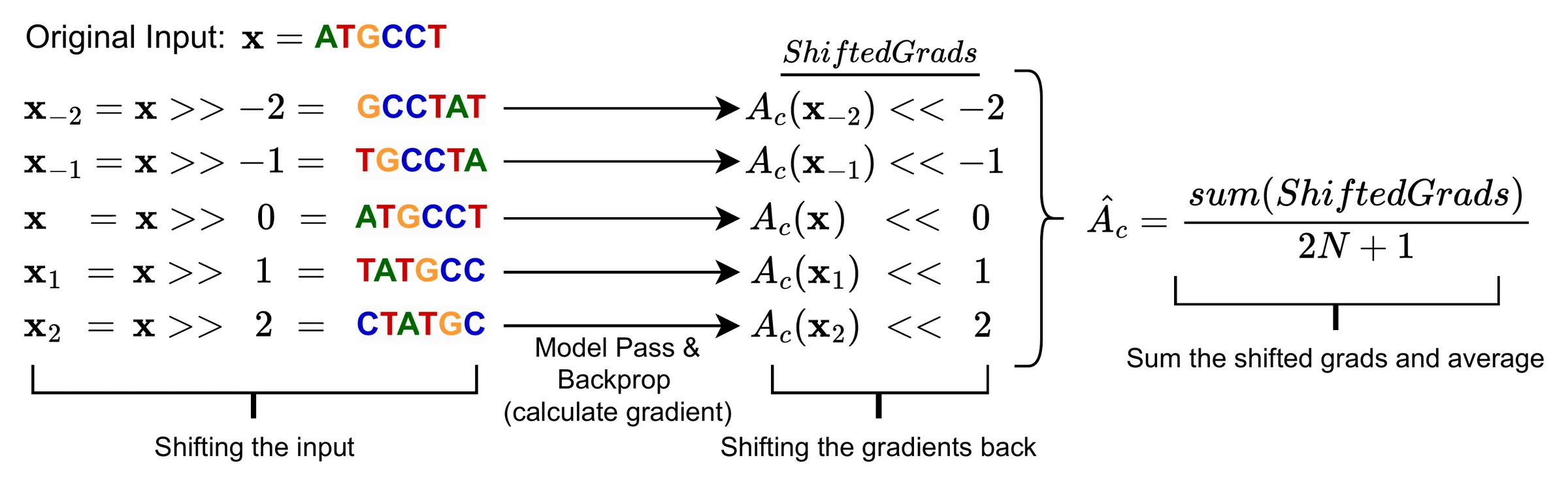
\hat{A}_c(x) = \frac{1}{2N+1} \sum_{n=-N}^{N} \mathrm{roll}\!\big(A_c(\mathrm{roll}(x,\, n)),\, -n\big), \qquad A_c(x) = \frac{\partial S_c(x)}{\partial x}

Diagram: the sequence ATGCCT is shifted by -2, -1, 0, 1 and 2 positions; each shifted copy goes through a model pass and backpropagation to give a gradient, each gradient is shifted back by the same amount, and the shifted gradients are summed and divided by 2N plus 1. — How ShiftSmooth works: the input is shifted by a small set of integer translations, a gradient is computed for each shifted copy, the gradients are shifted back to the original nucleotide positions and then averaged. Every shifted input remains a valid one-hot sequence, so the average stays on the data simplex. Reproduced from Tripathi et al. (2026), *Mathematics*, CC BY 4.0.

Every shifted copy is still a valid one-hot sequence, so, unlike Gaussian smoothing, the average stays on the data simplex. For the mixture, we take the derivative of the HetMoE output with respect to the single input tensor shared by all convolutional experts, so the map explains the whole model.

Data and evaluation

The experts and gate are trained on seven ENCODE ChIP-seq factors, each from a different DNA-binding-domain (DBD) family: ARID3A, FOXM1, GATA3, JUND, MAX, GABPA and SP1. Four of the seven training factors, and most of the held-out factors, come from the K562 cell line, so that the train/test boundary is not also a cell-line boundary.²

The held-out factors are split into three strata, each reported on its own:

Within-family (17 factors). Untrained members of the trained families, such as JUN and FOSL1 for JUND, MYC and USF1 for MAX, and GATA1 and GATA2 for GATA3. This stratum tests motif-family transfer.
Cross-family (6 factors). Sequence-specific factors from families absent in training: CTCF, STAT3, NRF1, HNF4A, TCF7L2 and ZBTB33.
Non-motif (6 factors). POLR2A, EP300, EZH2, TAF1, RBBP5 and SAP30. These are reported separately and never folded into the headline mean.

The headline OOD number is the mean over the 23 motif-bearing factors (within- plus cross-family). Experts train on GC- and repeat-matched real genomic negatives sampled from hg19. A simple dinucleotide detector separates shuffled negatives from genomic ones at AUC 0.73 with matched GC content, which confirms that the shuffling artifact is learnable. Every model is scored on balanced curated test sets of 500 bound and 500 unbound sequences per factor, with deterministic inference and a B = 1000 paired bootstrap (the same resamples for all models), plus a one-way ANOVA as an omnibus check. Pool and gate settings are chosen on in-distribution mean AUC only, and the OOD strata are scored once.

Results

In-distribution mean AUC, 7 training factors: 0.881
Motif-OOD AUC over 3 seeds (DNABERT-6: 0.799 ± 0.008): 0.821 ± 0.005
Motif-bearing OOD factors where HetMoE beats DNABERT-6 (95% CI, canonical seed): 13 of 23
AUC from gating over a static average of the same experts (canonical seed): +0.073

HetMoE has the highest in-distribution mean AUC (0.881) and the highest per-factor mean on all seven training factors, tying the fine-tuned DNABERT-6 on MAX. On the held-out factors it leads every motif-bearing stratum. On the separately reported non-motif stratum, which sits near a sequence-only ceiling, DNABERT-6 is the stronger model (0.756 vs 0.696).

Model	In-dist.	Within-family	Cross-family	Non-motif	Motif-OOD
HetMoE	0.881	0.846	0.775	0.696	0.827
DNABERT-6 (fine-tuned)	0.818	0.816	0.753	0.756	0.800
DanQ	0.827	0.805	0.746	0.702	0.789
DeepSEA	0.805	0.792	0.724	0.693	0.774
Static average of pool	0.796	0.770	0.707	0.675	0.754
Best single expert	0.747	0.754	0.693	0.654	0.739

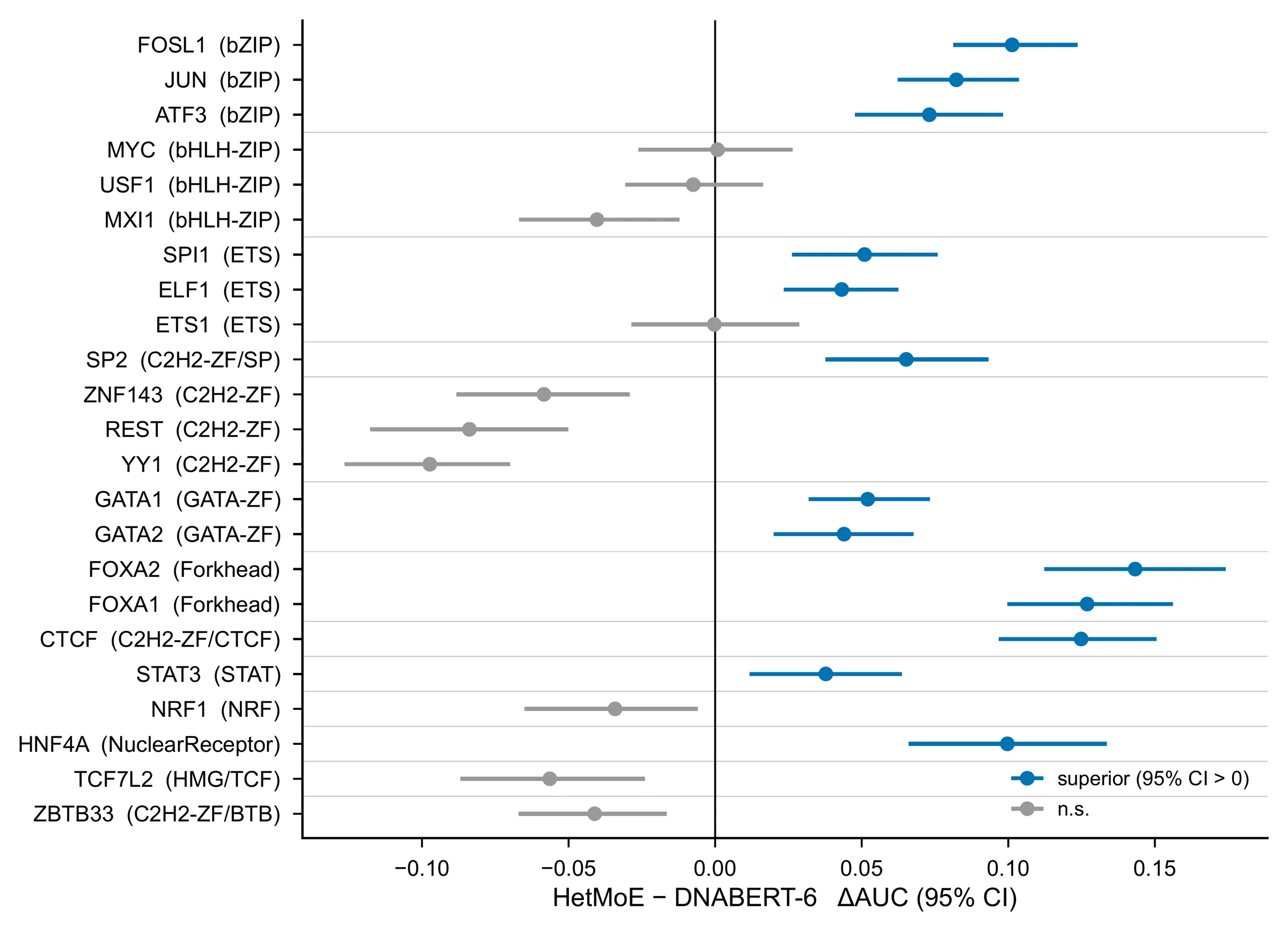
Mean AUC per stratum on the canonical seed (paper Table 3). Baselines are mean-ensembled across the seven training factors. All experts are trained on GC-matched genomic negatives. Best value per column in bold.

Against DNABERT-6, the per-factor paired bootstrap finds HetMoE significantly better on 13 of the 23 motif-bearing factors: 10 of 17 within-family (mean margin +0.029) and 3 of 6 cross-family (+0.022). The largest gains are on sequence-specific factors: FOXA2 (+0.143), FOXA1 (+0.127), CTCF (+0.125), FOSL1 (+0.101) and HNF4A (+0.100). On several zinc-finger factors (YY1, ZNF143, REST and ZBTB33), DNABERT-6 is stronger. Once the shuffle artifact is removed, these are the factors where genome-scale pretraining helps most.

Forest plot of HetMoE minus DNABERT-6 AUC difference for 23 held-out factors. Blue points with intervals above zero (significant) include FOSL1, JUN, ATF3, SPI1, ELF1, SP2, GATA1, GATA2, FOXA2, FOXA1, CTCF, STAT3 and HNF4A, with FOXA2 largest near 0.14. Grey points, which do not favor HetMoE, sit near zero for MYC, USF1 and ETS1 and below zero for MXI1, ZNF143, REST, YY1, NRF1, TCF7L2 and ZBTB33. — Per-factor HetMoE minus DNABERT-6 ΔAUC with 95% paired-bootstrap confidence intervals for the 23 motif-bearing held-out factors, grouped by DNA-binding-domain family. The interval excludes zero in favor of HetMoE on 13 of the 23 factors (blue), with the largest gains on FOXA2, FOXA1, CTCF, FOSL1 and HNF4A. Reproduced from Tripathi et al. (2026), *Mathematics*, CC BY 4.0.

Across random seeds

Each seed retrains every expert on the genomic negatives and reselects the configuration on in-distribution AUC. All three seeds select the same convolutional pool. The HetMoE margin over DNABERT-6 is positive in every seed (range +0.011 to +0.028), and HetMoE is also the more stable model (s.d. 0.005 vs 0.008).

HetMoE
Baselines

HetMoE± 0.0050.821

DNABERT-6± 0.0080.799

DanQ± 0.0060.782

DeepSEA± 0.0030.774

0.70.85

Motif-OOD mean AUC (3 seeds)

Motif-bearing OOD AUC, mean over three genomic seeds (paper Figure 5). Error bars are omitted; standard deviations are listed next to each label. The axis starts at 0.70.

Gating versus pooling

A gate over the seven ConvNet experts alone generalizes poorly (0.673). Adding the DeepSEA and DanQ trunks lifts the motif-OOD mean to 0.827, and in-distribution AUC selects that configuration. Adding fine-tuned DNABERT-6 experts as well (the full 28-expert pool) does not raise the mean any further (0.818), so the selected pool contains no genomic language model. Removing the two gate stabilizers lowers performance and collapses the gate’s mean entropy from 2.87 to 0.98 nats, concentrating it on a handful of experts.

ConvNet only7 experts0.673

DNABERT-6 only7 experts0.725

ConvNet + DNABERT-614 experts0.743

ConvNet + DeepSEA + DanQ (selected)21 experts0.827

Full pool, with DNABERT-628 experts0.818

Full pool, no stabilizers28 experts0.800

0.60.85

Motif-OOD mean AUC

Motif-bearing OOD mean AUC by expert pool, under the fair-negative protocol (paper Table 6). The note under each label gives the number of experts. The axis starts at 0.60.

Heatmap of mean gate weight, 0 to about 0.14, with rows JUN, MYC, ELF1, SP2, GATA2 and CTCF and 21 columns for the ARID3A, FOXM1, GATA3, JUND, MAX, GABPA and SP1 experts of each of ConvNet, DeepSEA and DanQ. Weight concentrates on different experts per row, for example DeepSEA-JUND for JUN, ConvNet-MAX for SP2, DanQ-GABPA for ELF1 and DanQ-FOXM1 for CTCF. — Mean gate weight for each expert in the selected pool (columns: the ConvNet, DeepSEA and DanQ experts for the seven training factors, grouped by backbone) across representative held-out factors (rows). The gate routes inputs in a factor-dependent way rather than collapsing onto a single expert. Reproduced from Tripathi et al. (2026), *Mathematics*, CC BY 4.0.

Negatives change the story

When the experts are instead trained against dinucleotide-shuffled negatives, the apparent motif-OOD margin over DNABERT-6 grows to +0.066 (mean 0.864, superior on 22 of 23 factors). Under fair GC-matched negatives it is +0.027 (mean 0.827, superior on 13 of 23). The common shuffle protocol materially overstates the comparison, so we report the fair-negative result as the headline.

ShiftSmooth in practice

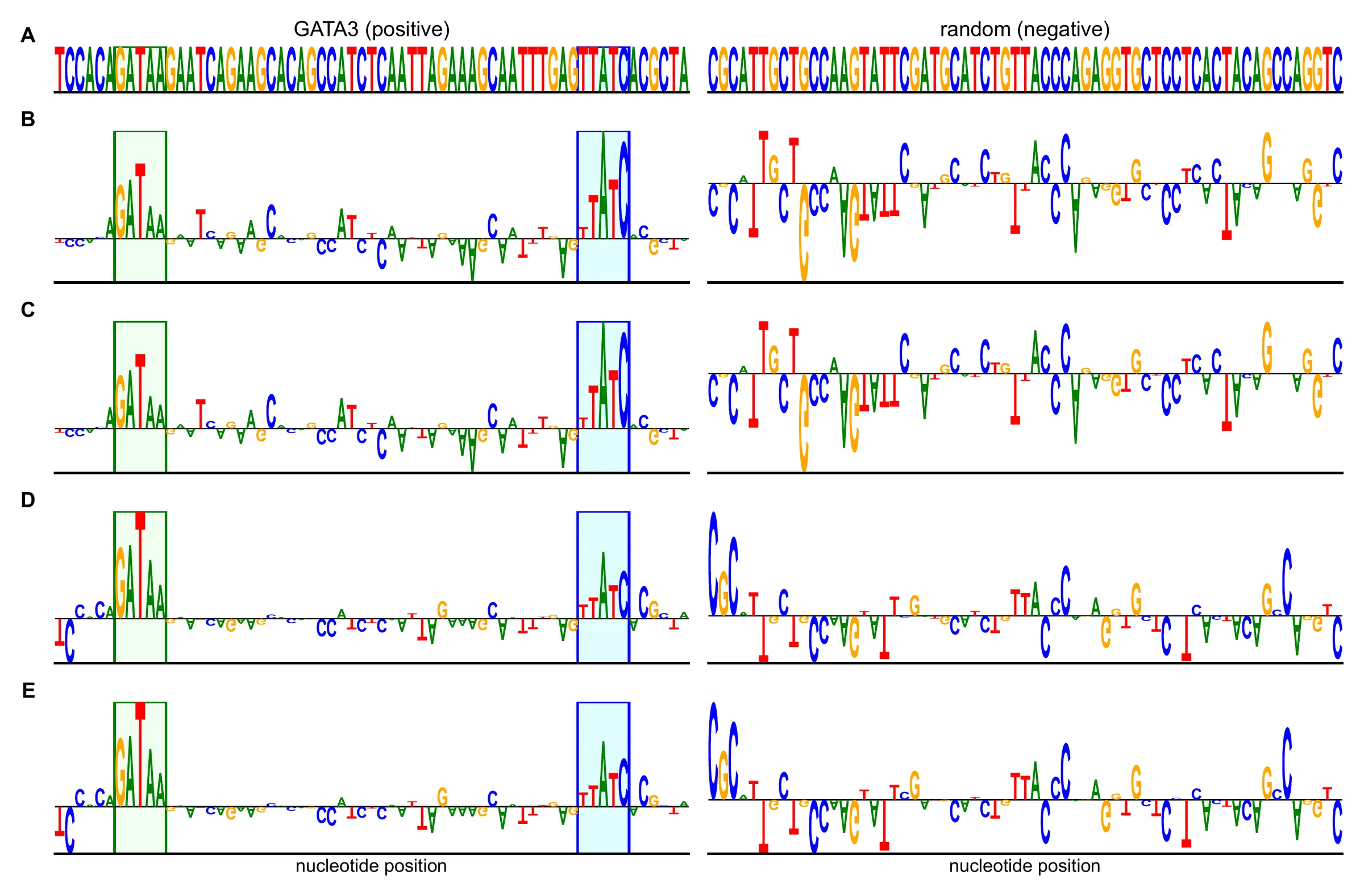
We compared ShiftSmooth with Vanilla Gradient, gradient × input and SmoothGrad on 50 positive sequences per training factor, with and without the simplex gradient correction of Majdandzic et al.⁷, for both the mixture and the individual experts. Faithfulness is rank correlation with in-silico mutagenesis; stability is attribution correlation under a small input perturbation.

Model	Method	Faithfulness	Stability
MoE	ShiftSmooth +corr	0.75	0.96
MoE	SmoothGrad +corr	0.76	0.92
MoE	Vanilla Gradient +corr	0.75	0.95
MoE	ShiftSmooth	0.72	0.96
MoE	SmoothGrad	0.75	0.92
Experts	ShiftSmooth +corr	0.78	0.95
Experts	SmoothGrad +corr	0.78	0.91
Experts	Vanilla Gradient +corr	0.78	0.95
Experts	ShiftSmooth	0.72	0.95
Experts	SmoothGrad	0.73	0.91

Attribution faithfulness and stability (paper Table 7). +corr applies the simplex gradient correction. Higher is better for both; bold marks the highest stability per model class.

ShiftSmooth with the correction matches or exceeds every other method on stability for both model classes (0.96 for the mixture, 0.95 for the experts), above SmoothGrad (0.92 and 0.91). Faithfulness is comparable across the corrected methods, and the simplex correction, not the smoothing kernel, accounts for most of the faithfulness gain. On a GATA3-positive sequence, Vanilla Gradient on the GATA3 expert gives the leading G of the GATAA motif almost no importance, while ShiftSmooth credits it. For the mixture, Vanilla Gradient gives the second A a negative score, which ShiftSmooth shows to be a window artifact: the same A scores positively once the sequence is shifted slightly.

ShiftSmooth attribution for a GATA3-positive sequence (left) and a random negative (right), zoomed to the motif region: (A) the input one-hot sequence, (B) Vanilla Gradient and (C) ShiftSmooth for the GATA3 ConvNet expert, (D) Vanilla Gradient and (E) ShiftSmooth for the MoE. The green box marks the GATAA motif and the blue box its reverse complement TTATC; letter height encodes per-nucleotide attribution in arbitrary units. Reproduced from Tripathi et al. (2026), Mathematics, CC BY 4.0.

What we learned

Key takeaway

The gain comes from per-input gating over complementary convolutional backbones, not from averaging more models or adding a genomic language model. The configuration chosen on in-distribution data alone contains no language model and still edges out a fine-tuned DNABERT-6 on the held-out motif-bearing mean, by a margin that is consistent across seeds but modest.

The evaluation protocol mattered as much as the architecture. An earlier preprint of this work⁸ gated pretrained CNN experts and tested on six randomly selected OOD factors, a set that mixed motif-rich and motif-free factors in one average. For the journal version we moved to seven training factors, family-stratified test strata and genomic negatives.

The paper also lists its limitations:

Generalization depends on motif family. Transfer is most reliable within a trained family (0.846). It is harder across families (0.775) and near a sequence-only ceiling for non-motif factors (0.696).
Cell-line and assay confounds. Anchoring to K562 reduces these but cannot fully exclude them.
Metrics and prevalence. AUC on a balanced 500/500 set measures ranking. It does not reflect deployment precision, where binding sites are rare.
Selection and scale. The selected configuration is the best of a small screened set and may be slightly optimistic. The study covers 7 training and 29 held-out factors over three seeds.
ShiftSmooth is not a faithfulness oracle. Its advantage lies in stability and on-simplex validity, not in beating corrected gradient baselines on faithfulness.

Where it goes next

A sequence-only predictor covers one regulatory modality. The paper’s stated next step is to fold explainable per-modality models like HetMoE into multimodal oncology pipelines that combine genomic, imaging and clinical data (MINDS).⁹ Foundation-model embeddings (HONeYBEE)¹⁰ and multi-omics networks (SeNMo)¹¹ offer one route, in which the same embedding gate could weight data sources the way it now weights experts.

Resources

Paper: open access in Mathematics (CC BY).²
Code: the tfbs library and the experiment command-line tools.¹²
Data: the processed ENCODE ChIP-seq sequences on Hugging Face (1,014 files).¹³
Weights: 7 ConvNet experts plus the DeepSEA and DanQ probes for seeds 0, 1 and 42.¹⁴

From the repository README (run from the repository root):

git clone https://github.com/lab-rasool/TFBS.git && cd TFBS
pip install -e .   # after installing the CUDA build of torch (see README)
hf download Lab-Rasool/ENCODE-TFBS --local-dir models   # checkpoints; ChIP-seq data go under data/

# HetMoE
python -m experiments.hetmoe.cache_embeddings --seed 42 --backbones ConvNet,DeepSEA,DanQ,DNABERT6
python -m experiments.hetmoe.sweep --seed 42
python -m experiments.hetmoe.aggregate_seeds

# ShiftSmooth attribution evaluation
python -m experiments.attribution.shiftsmooth_eval --n_seqs 60

Alipanahi B, Delong A, Weirauch MT, Frey BJ. Predicting the sequence specificities of DNA- and RNA-binding proteins by deep learning. Nat Biotechnol. 2015;33:831-838. doi:10.1038/nbt.3300 ↩
Tripathi A, Nielsen IE, Umer M, Ramachandran RP, Rasool G. Robust Transcription Factor Binding Site Prediction and Explainability Using a Heterogeneous Mixture of Experts Architecture. Mathematics. 2026;14(14):2489. doi:10.3390/math14142489 ↩ ↩² ↩³
Ji Y, Zhou Z, Liu H, Davuluri RV. DNABERT: pre-trained Bidirectional Encoder Representations from Transformers model for DNA-language in genome. Bioinformatics. 2021;37:2112-2120. doi:10.1093/bioinformatics/btab083 ↩
Tourne N, De Waele G, Vermeirssen V, Waegeman W. How negative sampling shapes the performance of transcription factor binding site prediction models. Bioinformatics. 2026;42:btag048. doi:10.1093/bioinformatics/btag048 ↩
Zhou J, Troyanskaya OG. Predicting effects of noncoding variants with deep learning-based sequence model. Nat Methods. 2015;12:931-934. doi:10.1038/nmeth.3547 ↩
Smilkov D, Thorat N, Kim B, Viégas F, Wattenberg M. SmoothGrad: removing noise by adding noise. arXiv:1706.03825, 2017. arxiv.org/abs/1706.03825 ↩
Majdandzic A, Rajesh C, Koo PK. Correcting gradient-based interpretations of deep neural networks for genomics. Genome Biol. 2023;24:109. doi:10.1186/s13059-023-02956-3 ↩
Tripathi A, Nielsen IE, Umer M, Ramachandran RP, Rasool G. Explainable AI in Genomics: Transcription Factor Binding Site Prediction with Mixture of Experts. arXiv:2507.09754, 2025. arxiv.org/abs/2507.09754 ↩
Tripathi A, Waqas A, Venkatesan K, Yilmaz Y, Rasool G. Building flexible, scalable, and machine learning-ready multimodal oncology datasets. Sensors. 2024;24(5):1634. doi:10.3390/s24051634 ↩
Tripathi A, Waqas A, Schabath MB, Yilmaz Y, Rasool G. HONeYBEE: enabling scalable multimodal AI in oncology through foundation model-driven embeddings. npj Digit Med. 2025;8:622. doi:10.1038/s41746-025-02003-4 ↩
Waqas A, Tripathi A, Ahmed S, et al. Self-Normalizing Multi-Omics Neural Network for Pan-Cancer Prognostication. Int J Mol Sci. 2025;26:7358. doi:10.3390/ijms26157358 ↩
lab-rasool/TFBS: code, training and evaluation pipeline. github.com/lab-rasool/TFBS ↩
Lab-Rasool/ENCODE-TFBS dataset (ENCODE ChIP-seq sequences). huggingface.co/datasets/Lab-Rasool/ENCODE-TFBS ↩
Lab-Rasool/ENCODE-TFBS model checkpoints. huggingface.co/Lab-Rasool/ENCODE-TFBS ↩